Justified Working Assumption: The Footage Shows External Objects, and not Effects of Light or Digital Processing
In the chapter about data reliability I present my arguments for the claim that the WFM phenomenon is about a real external physical phenomenon and not a result of a fabricated hoax or confounding factors from a mundane source. “External” means that WFM footage is caused by a genunine unknown physical source outside of the camera device or any process of ex-post image alteration. In summary, the best video footage of WFM show some or all of the following features that support this view:
Footage is unsensational and unsensationally presented
Phenomenon is very stable under a vast variety of pluralistic data sources (i.e. individuals with very different social backgrounds, technically diverse video equpiment)
No or only weak personal gain from hoaxed uploads
Originators are technically incapable of hoaxing footage
Phenomenon occurs accidentally in other video footage without being specifically pointed out
Despite the phenomenons stability (b), captures show diverse viewing angles and flying patterns that are consistent with intentional steering
Footage is consistent with expectations given the differences in the described technical equipment
Data is not consistent with any mundane explanation of lens glares, insects, birds or any other known effects or objects
See my chapter about data reliability for further details. We use this claim as a working assumption for further video analysis of the available footage. This analysis is aimed at getting a better understanding of WFMs flight patterns, i.e. their flight trajectories and speed.
Estimation of Travel Speed
Humans are well equipped for interpreting distances and movement speeds of the objects they see in their environment. This proposition can be supported by the simple fact that only these capabilities make it possible to play Tennis, Football, Baseball and the likes. This proposition may also be substantiated by reference to evolution theory; we, such as many other mammals, need these capabilities to survive in an environment filled with hunters and pray.
However, optical illusions can make us misinterpret visual data. Furthermore, an analysis of a video from one optical lens does not provide the important information of different viewing angles for the estimation of distances and speed—that is why mammals use two eyes. In the following I show, firstly, that our visual intuitions, as well as a methodological analysis, let us estimate WFMs' movement speed to be usually in the ballpark of an order of magnitude faster than objects like golf balls or common model planes. Secondly, I substantiate this first impression as being valid by a technical analysis that includes (i) the objects possible trajectory, (ii) the smear effect due to an extended shutter time at filming extremely fast objects, and (iii) the increase of the object's size in the image.
This estimation is aimed to provide very rough results to show that WFMs are very extreme phenomena that cannot be easily explained with mundane approaches (e.g. objects carried by wind, projectiles, drones). It is not crucially relevant to this result if we can estimate the traveling speed only very roughly, meaning that it might be off by ±30%. But it would be important if the estimation is off by a factor of 10. Therefore, the chosen methodology is aimed to provide reliable, rough and pragmatic results.
The following figures 1, 2 and 3 show three cases for the reader to compare regarding the visual intuition that they induce. Despite the very differing angles, a human observer has very clear intuitions about the object's travel path and approximate speed.
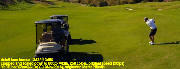
Fig 1. Professional golfer almost hits camera with long shot. The ball's average speed is about 172 km/h over a distance of around 185 meters. (original video)
Fig 2. Possible WFM with average speed of about 441 km/h. For analysis see case's analysis page.
Fig. 3. Possible WFM with average speed of about 2600 km/h. For analysis see case's analysis page.
Even significantly faster cases of WFMs than the one showed in figure 3 were measured, but the small number of frames and the strong smear effect (e.g. Sion, 13 Nov 2015) or the great distance of the object (e.g. Maryland Point, 12 Dec 2015) make them unsuitable cases for this introduction of the methodology.
This is how I estimate average speeds. In the first example we know the distance that the ball travels. Figure 4 illustrates this distance (185m) on satellite images from the original golf course. Furthermore, we know the frame rate of the video (30 frames per second) and that an hour has 60×60=3600 seconds. The golf ball's average traveling speed is
[distance travelled] / [number of frames with object flying] × [frames per second] × 3600,
which is for this example
0.185 km / (405-289) × 30 × 3600 × 1/h ≈ 172 km/h.
Speed estimates for the possible WFMs in figures 2 and 3 employing this methodology are given on their case pages as linked in the captions.
Fig 4. Estimate of ball's travelled distance with satellite imagery. (2012 WGC-Cadillac Championship at the Golf Resort & Spa in Doral, Florida. Google Maps link)
In the case from figure 1 we know the ball's travelled distance for certain, because we know where the tee is put and were the camera is located. For the cases of the WFM we only know that well were the camera is located, but we have to make a rough estimation of the WFM's positions based on the provided video data. The crucial assumption is that the object travels on a roughly constant altitude over the ground. Different viewing angles of several WFM cases strongly suggest this movement behavior. I defend this claim further in section (i) and (iii) below. Under this assumption an estimate of the distances can be provided for many cases of possible WFMs.
(i) Linear Trajectories, Most Often with Constant Altitudes
Strictly speaking, the patterns we see in WFM footage could be the result of something that moves very close to the lens with much lower speed and changing altitude. An insect is a candidate for producing such a confounding factor. However, this possibility is very unlikely due to the fact that the majority of very clear possible WFM footage is consistent with either a constant altitude of travel (most cases) or a steep linear ascension or descension. Figures 5 and 6 illustrate a simplified scenario in which the object may approach the drone with a linearly constant (path A) or changing (path B) altitude.
I defend that many cases of WFM footage indicate a constant altitude, which is then taken as a necessary assumption to estimate the traveling speed.
Fig. 5: Two possible paths to produce a video with an approaching object under the drone from the distance (assuming an indistinct change of the object's size in the image).
Fig. 6: Above view of the situation described by figure 1.
Figure 7 shows a list of examples with clearly identifiable travel paths of possible WFMs. For the analysis I mark the object's position in every frame, or at least in every nth frame with a fixed natural number n for each case, for practical reasons for footage with a very high framerate. If the camera is not sufficiently stable during the filming, I apply video stabilization routines. The trajectory analyses substantiate the hypothesis of WFMs often travelling at a constant altitude because we can observe many cases of flight patterns from very different angles that are very consistent with this assumption.
I use the geometry simulation software POV-Ray to replicate the footage of case 6BUA6zdbgEE. This replication validates the assumption of the WFM's roughly constant travel altitude for this case. Note that further unknown parameters are crucial to replicate the image perfectly, particularly the drone's and the object's specific altitude over the ground.
Fig. 8. Case 6BUA6zdbgEE (left), POV-Ray replication (right, source script), and overlay (bottom).
The path analyses summarized in figure 7 show all 4-5 star examples of possible WFM. Some noticeable characteristics of WFM can be derived: no erratic movements, almost linear travel paths or high-radius curves. Some examples indicate a clear change of altitude, and for many examples the altitude cannot be derived reliably.
(ii) Smear Effect due to Long Shutter Time
Film cameras as well as digital cameras need a certain amount of time to save the incoming image. This exposure time for film cameras is necessary for the chemico-physical process to engrain the image into the negative. Despite the purely electronic mechanism, digital cameras also need an extended period of time to capture enough incoming light to detect an image. This period also depends on the intensity of the incoming light (less light leads to an increase of shutter time). With reference to a mechanism to suppress incoming light (shutter) into the camera lens this time frame is often called shutter speed or shutter time in digital imaging. I prefer the name shutter time, because, strictly speaking it refers to a time frame measured in (milli)seconds.
Figure 9 shows how objects that move significantly during the shutter time appear smeared in the finished picture.
Fig 9. Smear effect from car lights with increased shutter time up to several seconds (left) and from rotor blades that move significantly during common cameras' shutter time of only milliseconds.
Shutter times of cameras vary significantly depending on the camera's specific purpose. Ultra high-speed cameras, for instance, have shutter times short enough to clearly capture a gun bullet in closeup images, as figure 10 shows. Short shutter times can be achieved with high sensor sensitivity and high intensity of light exposure. Everyday camera equipment of drones or cellphones has significantly longer shutter times due to cost efficient hardware choices.
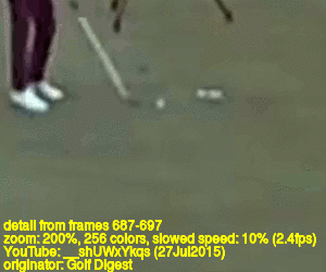
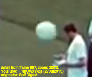
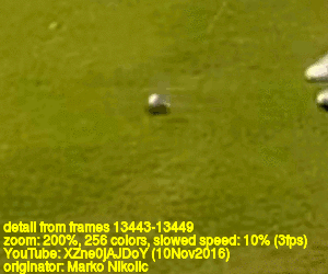
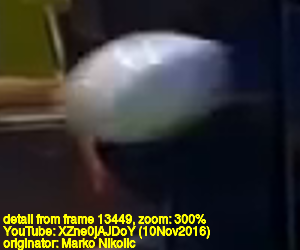
With focus on the topic of the web site it is most interesting how the cameras perform that were used in the actual cases. Not the absolute speed of an object is relevant, but the speed in the lens' view, which increases with the object's speed and decreasing distance to the lens. Figure 11 shows commonly used but slightly outdated equipment with white fast moving objects in front of their lense. As expected, the golf ball and the hail stones show smear effects when they are very close to the lens.
(click images to start/stop animation)
Fig 11. Enlarged and slowed view on near golf ball from figure 1 (left). A drone with a GoPro Hero 3 camera in a hail storm (right, original video).
It is crucially important to note that more recent drone models use very significantly improved optical sensors with highly decreased shutter times. I found some footage from golfers who try to hit recently produced (June 2018) drone models that are often used for the cases of possible WFM on this web site. As it turns out, see figures i and j, in bright sun shine the golf ball can be see extremely clear and without much smear, even if it passes the drone very closely and directly after the tee. We cannot estimate the exact approaching speed of the ball but it is apparent that the modern digital cameras have a very significantly shorter shutter time than the older but professional camera from the case of figure h, left. In standard configuration the drone cameras use the shortest possible shutter time. However, we need to be aware that the shutter time can also be manually increased to produce effects like the ones shown in figure 9—or to let an object appear faster in a photograph.
(click images to start/stop animation)
Fig 12. Professional golfer aims for a DJI Phantom 3 Standard and misses only barely. Scene with real speed (top), slowed version of flight (left), and closeup of ball in the last frame. (original video)
(click images to start/stop animation)
Fig 13. Amateur golfer aims for a DJI Mavic Pro and misses only barely. Scene with real speed (top), slowed version of flight (left), and closeup of ball in the last frame. (original video)
Note that the drones models in figure 12 an 13 are not models using camera sensors with particularly short shutter times (i.e. from the Sony Exmor series). These models use the Panasonic Smart and an undisclosed likely non-brand CMOS sensor which perform worse in benchmark comparison tests. See table 1 in chapter Reliability of WFM Data and Justified Inferences.
I conclude the following from this review of smear effects in general and in particular for the employed cameras of possible WFM footage:
Only an object with extremely high speed in front of the lens can produce a smear effect when captured with the most capable sensors, e.g. from the Sony Exmor series
The appearance, in particular the length, of the smear effect can vary significantly depending on the technical capabilities of the optical sensors, settings and lighting conditions
A false positive signal of a supersonic WFM could be fabricated but demands some specific finesse.
by filming a not so fast white object (e.g. a white model plane), chose an artificially long shutter time and increase the frame rate. However, this easy way of hoaxing data could be detected by the distorted movement patterns of other objects in the video (e.g. cars, birds)
Overall, the smear effect is a valuable feature of possible WFM footage to assess its reliability. It is not trivial to fabricate and depends on more than one factor.
The actual shutter time of taking a digital photograph depends on the specific lighting conditions. Using the same camera under the circumstances it was designed for the following rule holds: The more light there is available, the shorter the shutter time is. In the chapter about data reliability, section b.3 I summarise the technical equipment used to capture the WFM footage collected on this website. Furthermore, there I list the actual smear effects found in the footage. On the sites about the specific cases, I detail how the smear effect occurs in the cases.
If the WFMs in the footage often travel roughly at a constant altitute, then the smear effects in the footage well corroborate the extremely high, often supersonic speeds derived by applying the methodology outlined above.
(iii) WFMs' Change in Appearance during Approach
An object's size in an image is inversely proportional to its distance from the camera lens assuming a fixed focal length, i.e.
object's size in image ∝
1
object's distance to camera lens
Unfortunately, in most or all cases of useful WFM footage the imaging resolution and other factors do not allow for reliable estimates of the objects' change in size from one frame to another. These other factors include foremostly changes in light reflections, artefacts from digital video compression and the smear effect discussed above.
Can the Camera Capture a Small Object From Such a Great Distance?
Another question regarding the estimation of a travelling speed by dividing the covered distance by the time of travel taken is whether the estimated distances are even feasible to be captured by the cameras used. Cases in which the object approaches from far away with a derived maximal distance in the first frame of visibility are listed in the following table.
Case (image resolution) Drone (Sony Exmor R sensor)
Tab 1. Selected cases with an estimated travelled distance of at least 1,000 meters.
The precise size of the WFMs remains a variable in the analyses, but a diameter of a couple of decimeters seems to provide a reasonable first guess prima facie. Note that the specific lighting conditions significantly influence the image quality in the samples listed in table 1.
I conduct a real-world test under realistic conditions to corroborate that the captured WFM footage can be produced by an object of the mentioned size. For this I look at spots where a high contrast object of comparable size can be filmed from various distances of a few kilometers. I look over a straightened river. Figure 14 shows, a series of bridges and a church perfectly line up over the Isar river with a distance up to almost six kilometers. Given table 1 above, we are particularly interested in the visible detail of the Isarwehr building viewed from each of the two bridges
Fig 14. Isar river and the four selected land marks. The land marks the following distances apart: MJ Bridge to JFK Bridge: 0.99km, JFK Bridge to Isarwehr: 1.58km, Isarwehr to StV Church 3.11km.
I made videos under favorable weather conditions from the John F. Kennedy Bridge and from the Max Joseph Bridge towards the Isawehr with the tower of the St. Valentines Church in the background. The videos were recorded on a cloud-free afternoon in April with 35% humidity, 1031hPa and weak wind. I use a 12.3 megapixel f/2.0 aperture Sony IMX377EQH5 camera (housed in a LG Google Nexus 5X mobile phone) from the Exmor R series. The high-quality sensors in DJI's Phantom 3 Pro and Phantom 4 Pro are from the Exmor R series, too. (see chapter on data reliability, section b.3). I take 4K UHD videos with a resolution of 3840×2160 pixels. Most of the analysed cases on this web site are YouTube uploads with 2160p (2560×1440 pixels) or 1080p (1920×1080 pixels) resolutions. Therefore, I also downsized the videos to this resolution and selected frames from the results. Note that the aim of this study is to show that the estimated distances for the WFMs are very well in the realm of realistic captures with the described video equipment. Different hardware and different software may produce different results but not to a degree that would undermine my reasoning. YouTube's compression algorithms add an additional layer of distortion.
Figure 15 shows the Isarwehr and the Church's tower on cloudy days. Given the size of the white objects in the image, determinable in satellite pictures, we can infer from how well they are visible in the images to how well WFM footage fits to .
This means that they must be well distinguishable from the darker part of the roof captured from each of the two bridges.
Fig 15. Isarwehr (top) and St. Valentin Church. (both images by Wikimedia). The Isarwehr's small four dormers are about 1.40m wide each, the Church's tower's width is about 4.30m.
The following figures 16 and 17 show the results for the two bridges as camera location.
Fig 16. Isarwehr and St. Valentin Church captured from John F. Kennedy Bridge. 2160p (top), doubled zoom crop from 2160p (bottom left) and 1080p (bottom right).
Fig 17. Isarwehr and St. Valentin Church captured from Max Joseph Bridge. 2160p (top), doubled zoom crop from 2160p (bottom left) and 1080p (bottom right).
The following table summarizes the size of comparison objects to produce the captured test footage.
Camera Position
Object
Compares to Object ⌀ in 1km Distance
Compares to Object ⌀ in 2km Distance
Compares to Object ⌀ in 3km Distance
JFK Bridge
Isarwehr Dormers
0.89m = 1.40m / 1.58
1.77m = 1.40m / 1.58 × 2
2.66 = 1.40m / 1.58 × 3
JFK Bridge
Church Tower
0.92m = 4.30m / 4.69
1.84m = 4.30m / 4.69 × 2
2.75m = 4.30m / 4.69 × 3
MJ Bridge
Isarwehr Dormers
0.54m = 1.40m / 2.57
1.09m = 1.40m / 2.57 × 2
1.63 = 1.40m / 2.57 × 3
MJ Bridge
Church Tower
0.76m = 4.30m / 5.68
1.51m = 4.30m / 5.68 × 2
2.27m = 4.30m / 5.68 × 3
Tab 2. Diameters of comparison objects to produce the same optical signal than my test footage.
These results corroborate that an object of a few decimeters in diameter would produce an only barely noticeable white dot in images under similar conditions. Table 1 shows that this fits to the measured signal despite remaining uncertainties due to the very different production factors (eps. lighting conditions) for the footage.


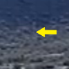
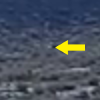
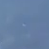
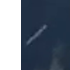
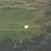
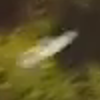
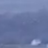
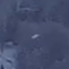
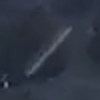
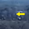
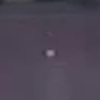
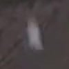
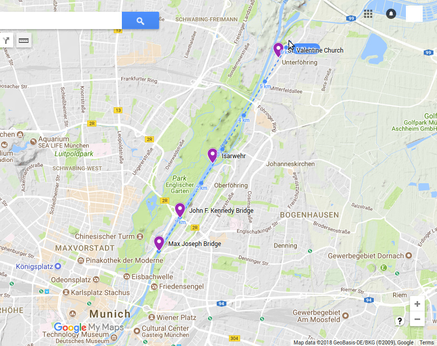 Fig 14. Isar river and the four selected land marks. The land marks the following distances apart: MJ Bridge to JFK Bridge: 0.99km, JFK Bridge to Isarwehr: 1.58km, Isarwehr to StV Church 3.11km.
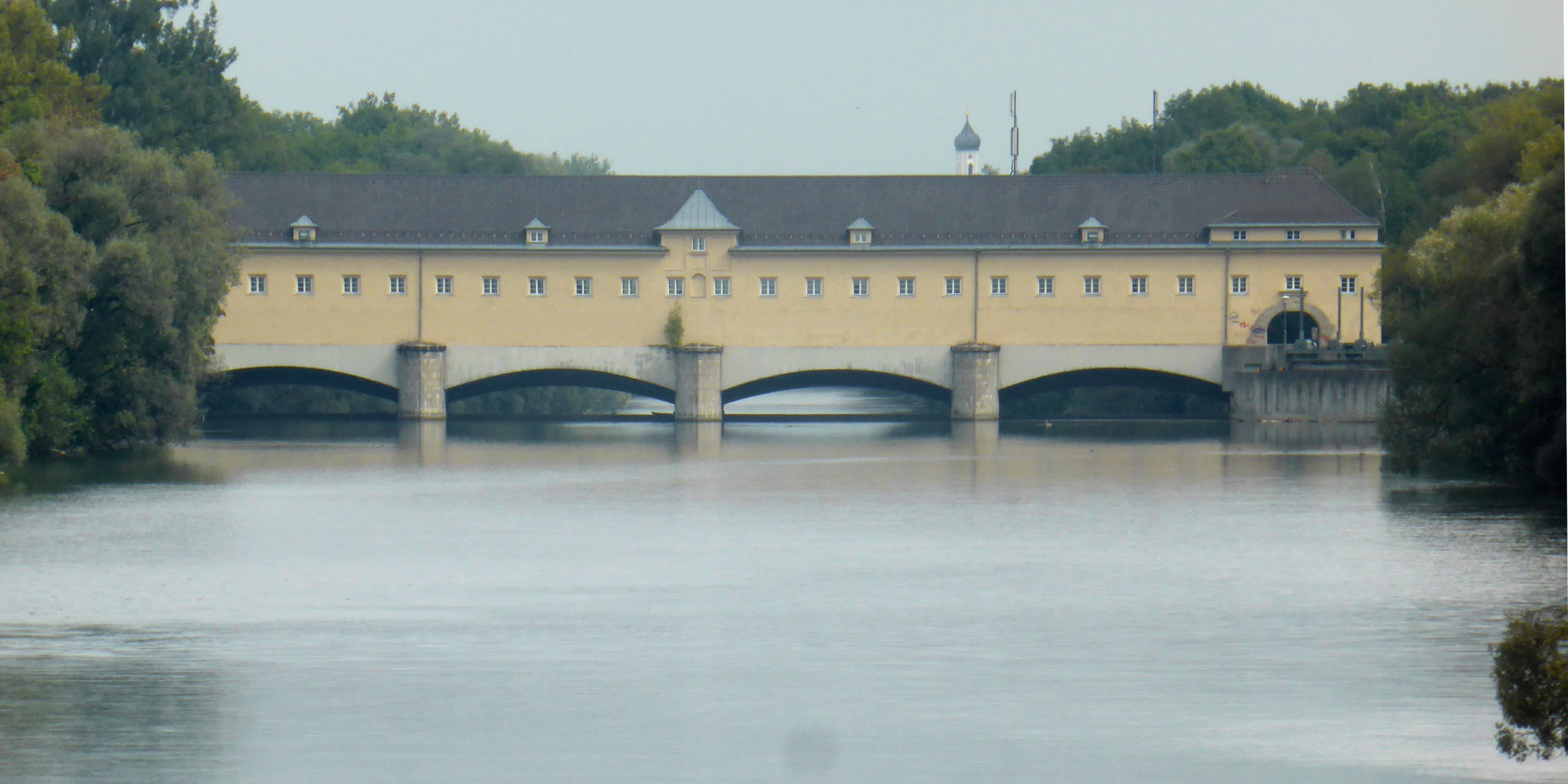
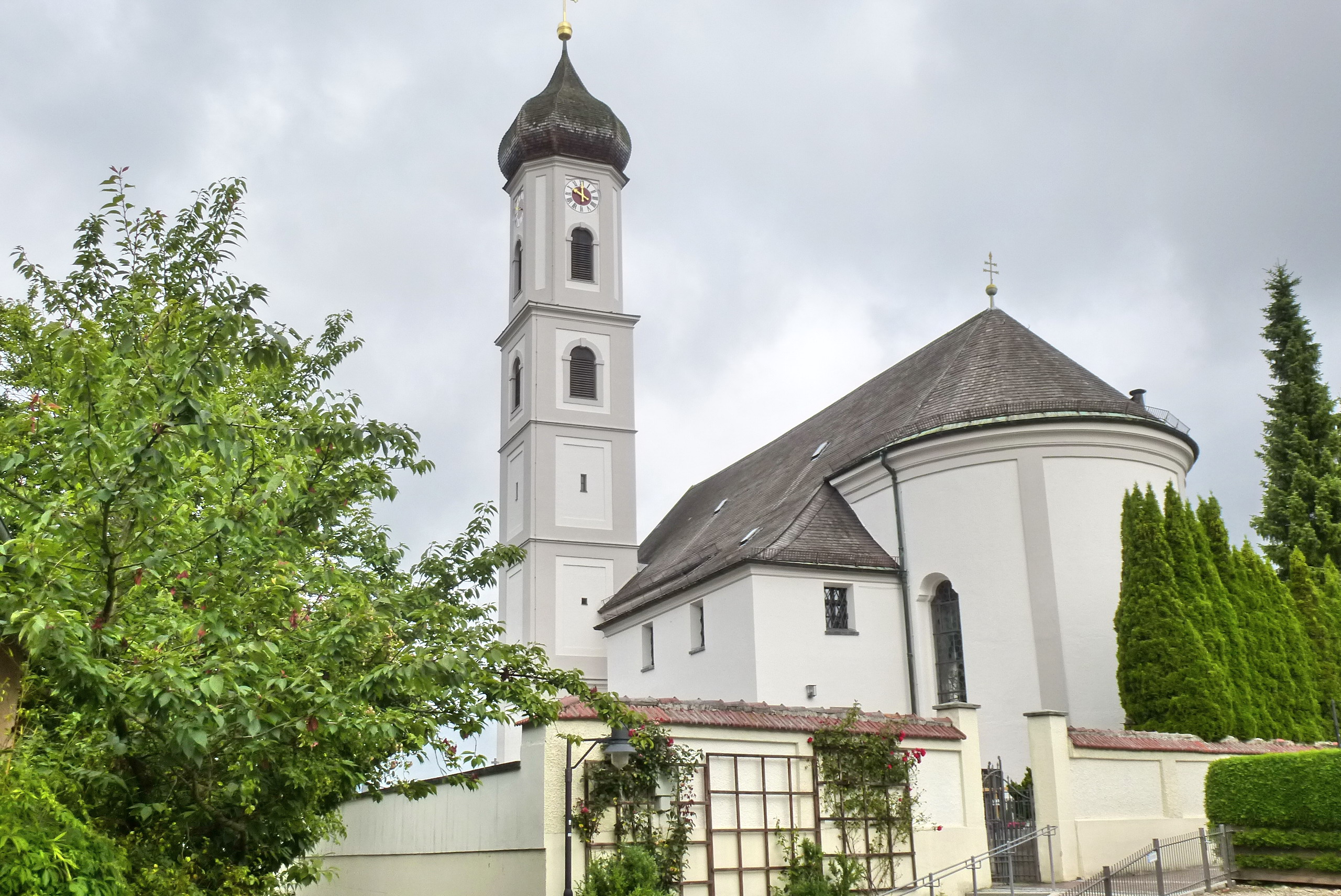
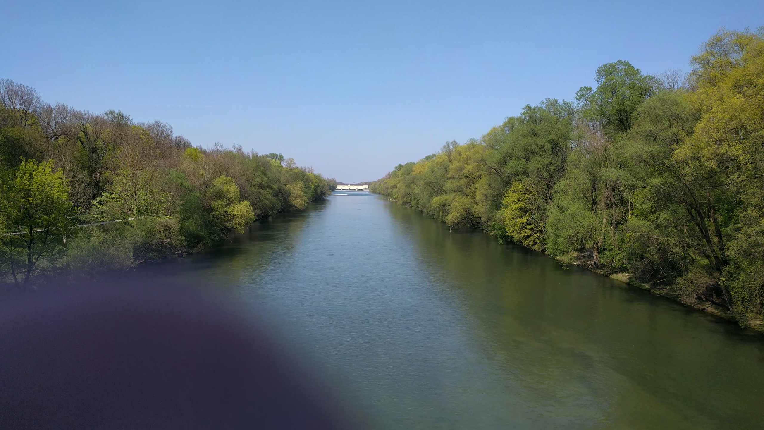
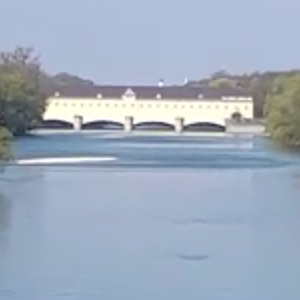
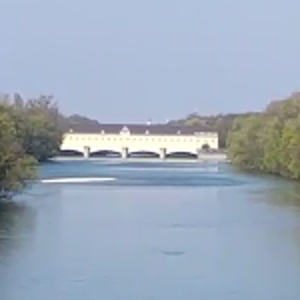 Fig 16. Isarwehr and St. Valentin Church captured from John F. Kennedy Bridge. 2160p (top), doubled zoom crop from 2160p (bottom left) and 1080p (bottom right).
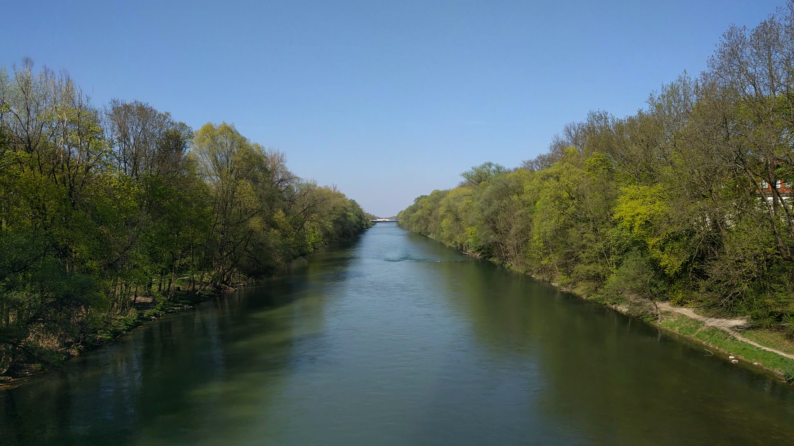
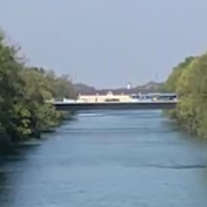
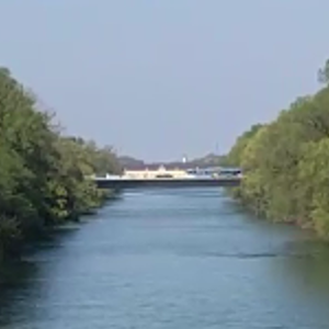 Fig 17. Isarwehr and St. Valentin Church captured from Max Joseph Bridge. 2160p (top), doubled zoom crop from 2160p (bottom left) and 1080p (bottom right).

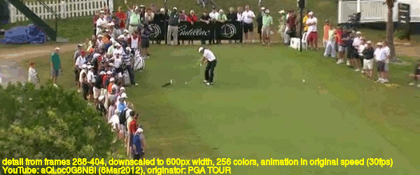 Fig 1. Professional golfer almost hits camera with long shot. The ball's average speed is about 172 km/h over a distance of around 185 meters. (
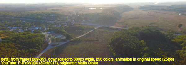 Fig 2. Possible WFM with average speed of about 441 km/h. For analysis see
 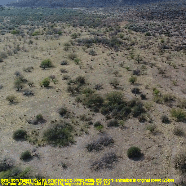 Fig. 3. Possible WFM with average speed of about 2600 km/h. For analysis see
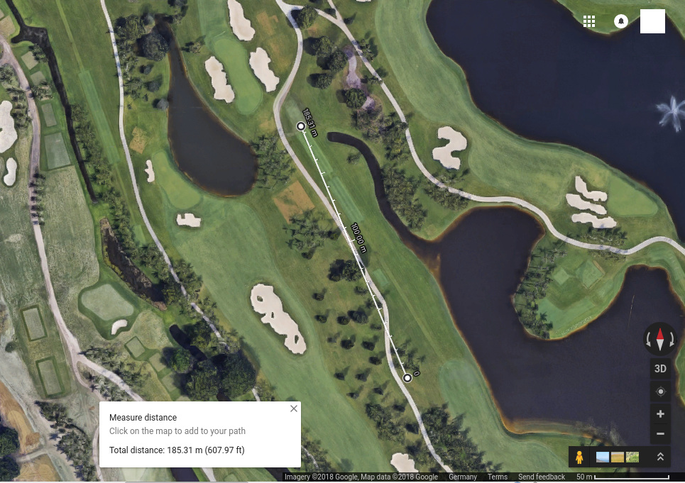
 Fig. 5: Two possible paths to produce a video with an approaching object under the drone from the distance (assuming an indistinct change of the object's size in the image).
 Fig. 6: Above view of the situation described by figure 1.
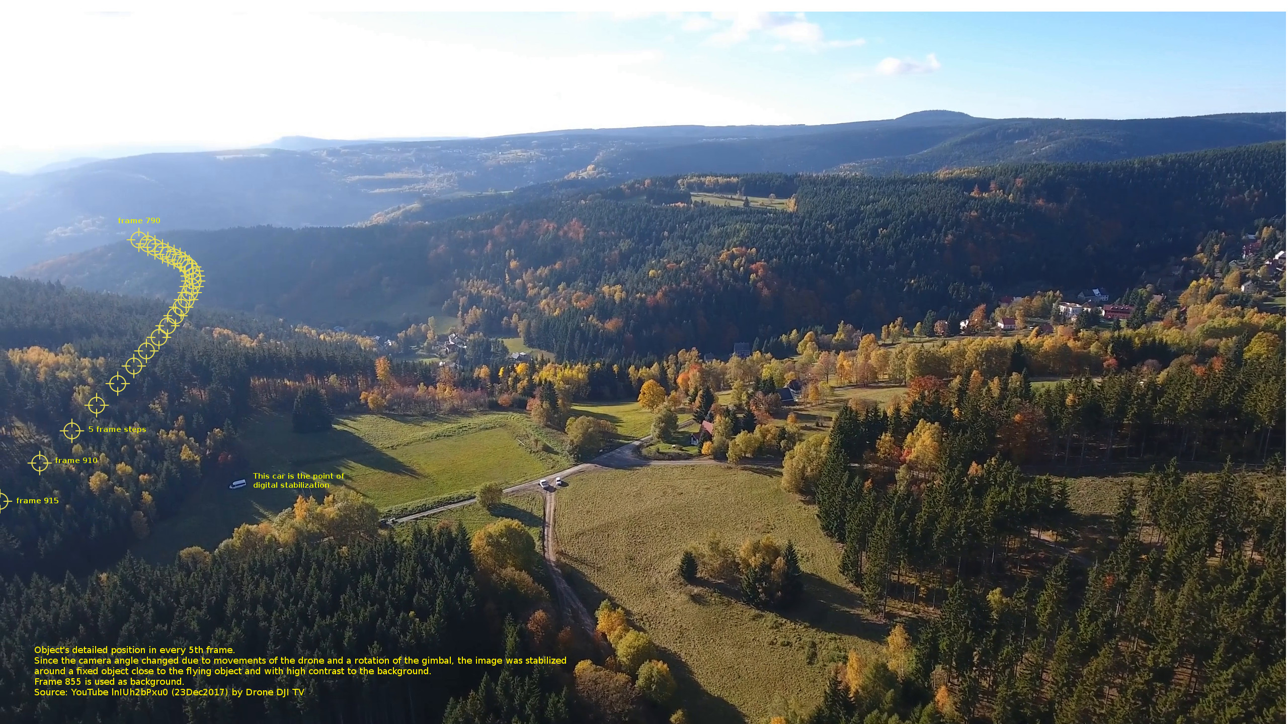
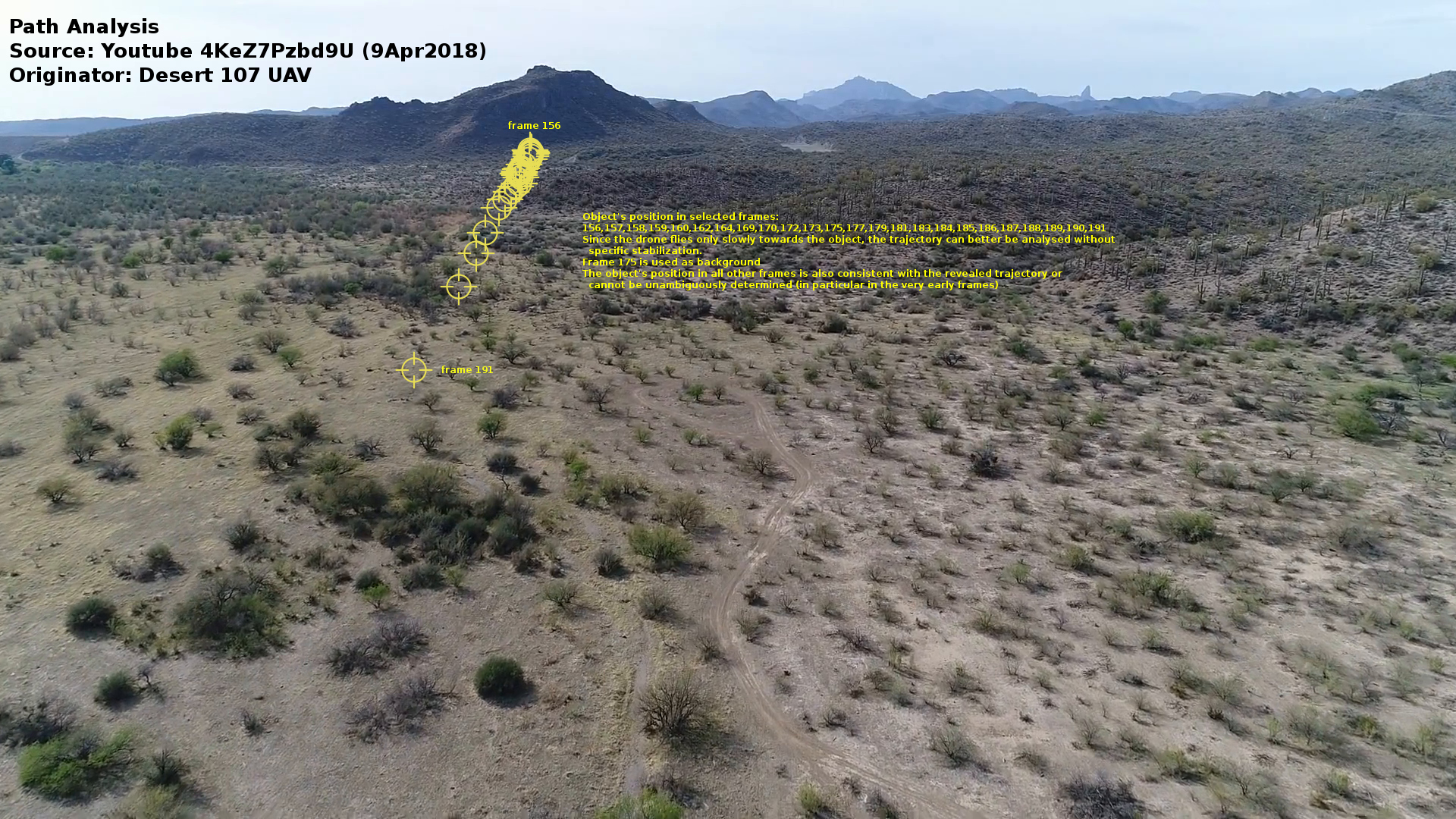
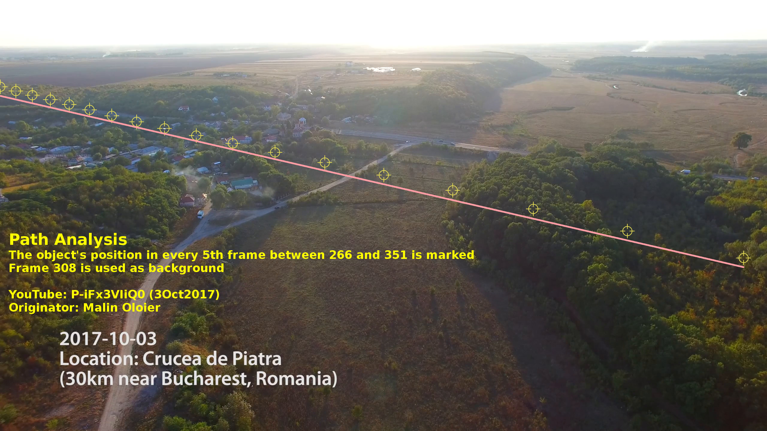
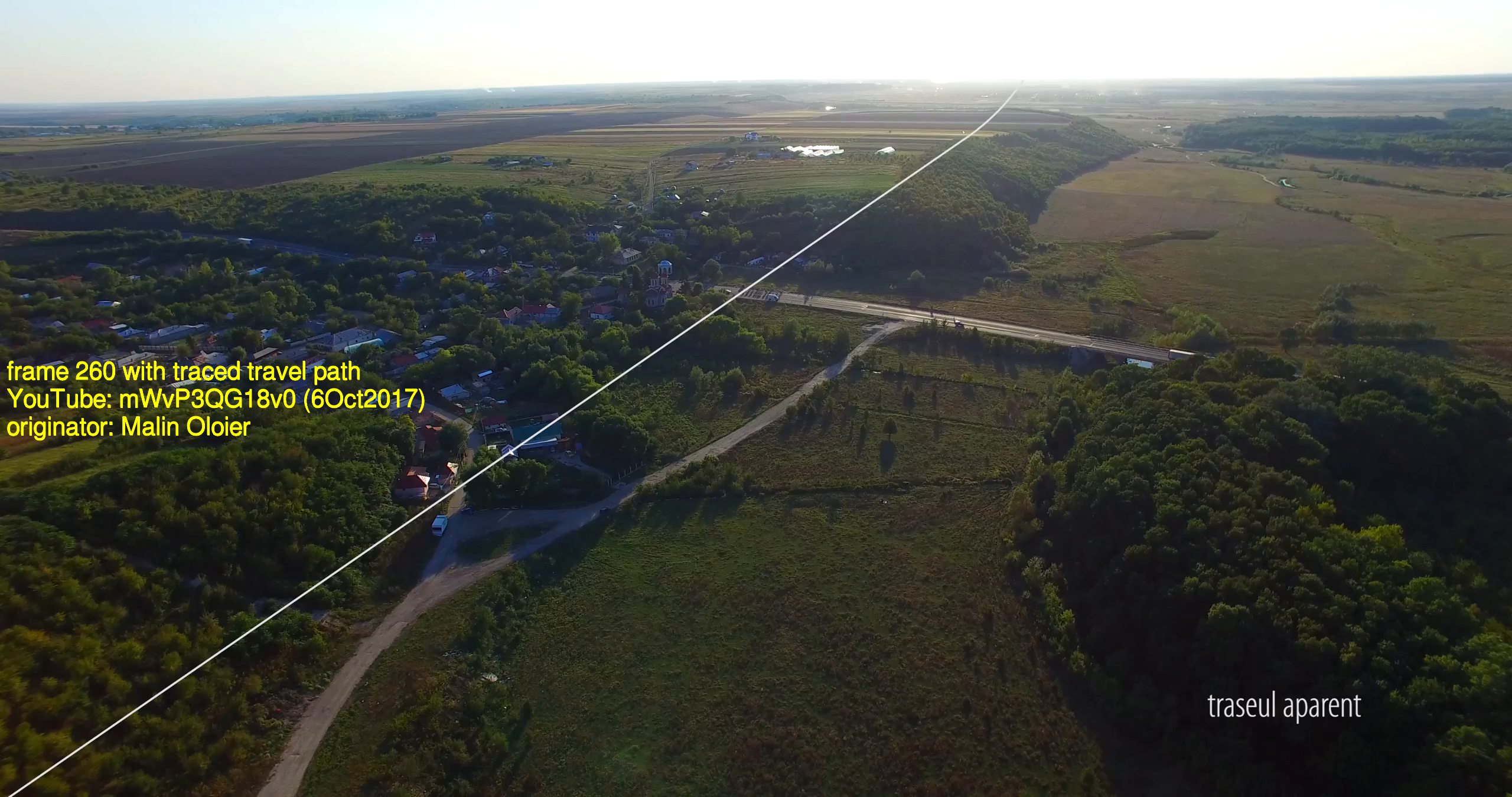
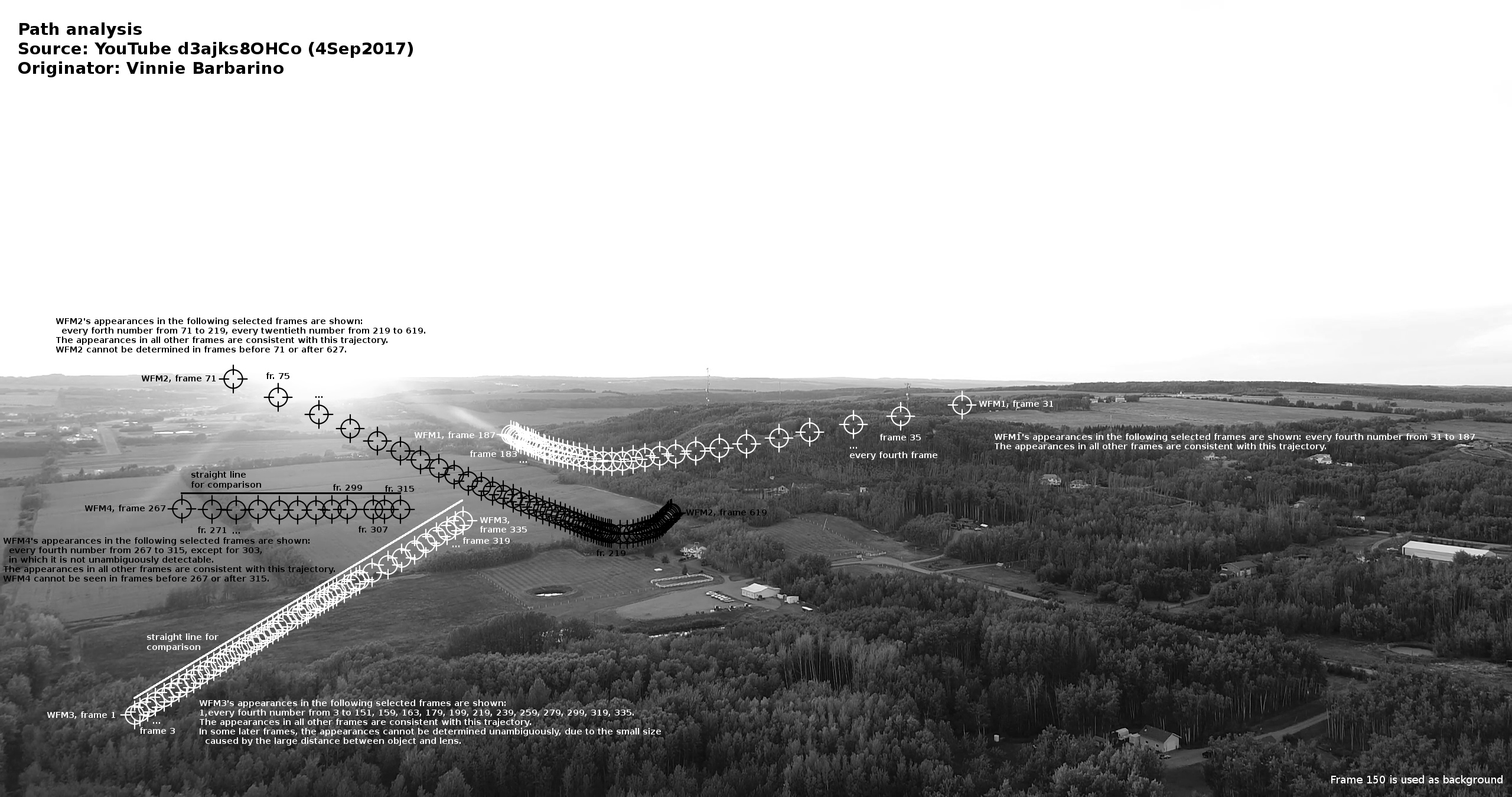
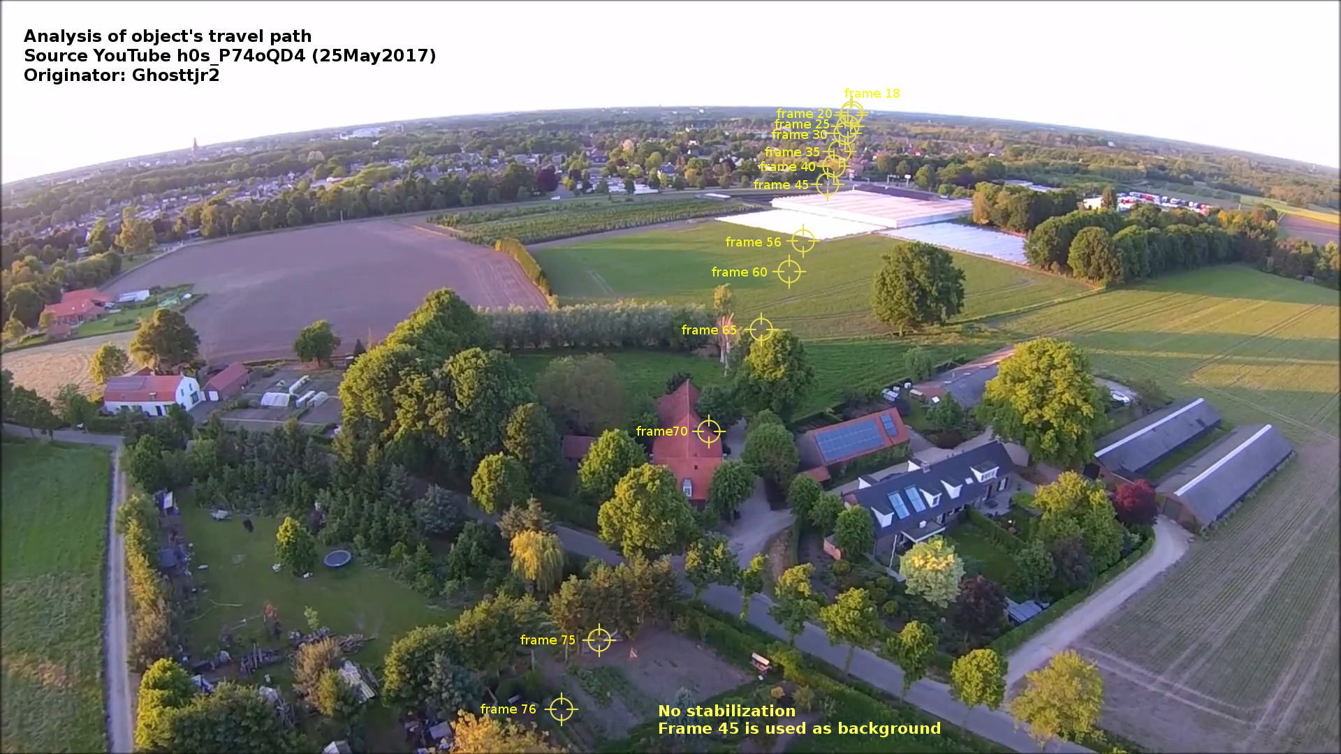
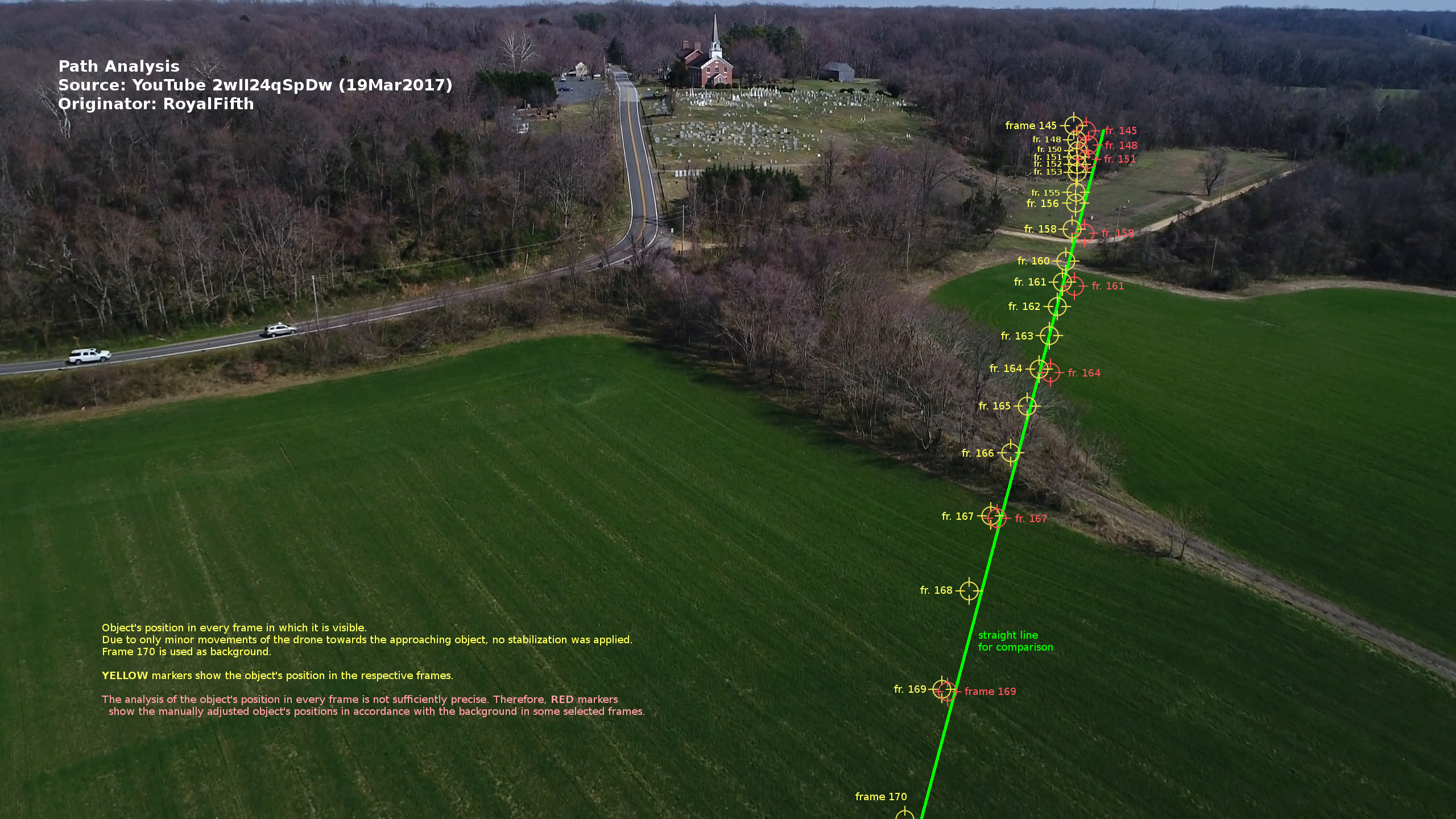
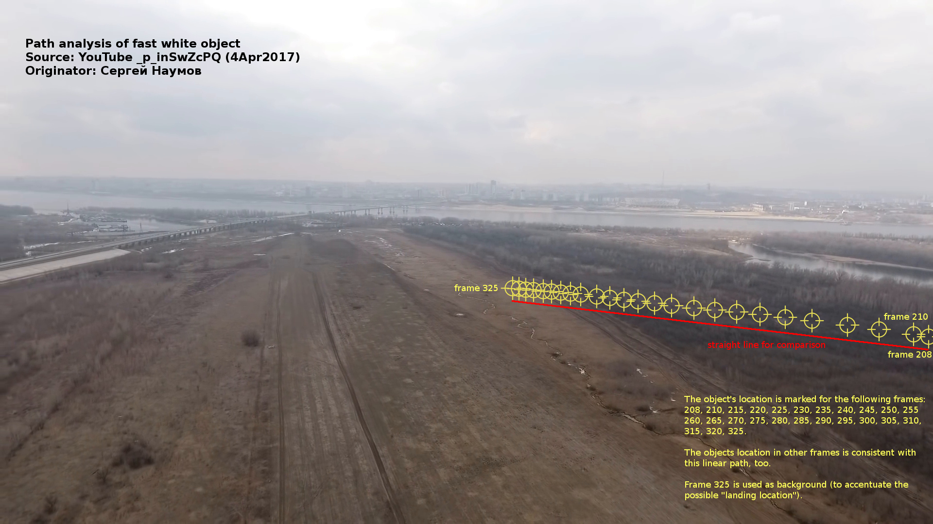
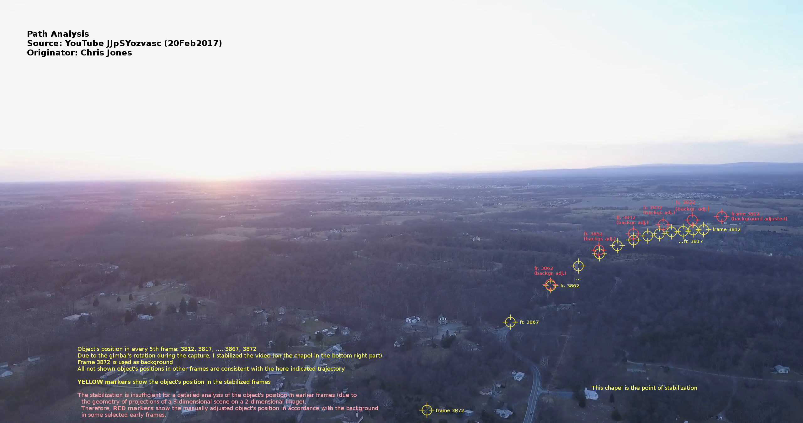
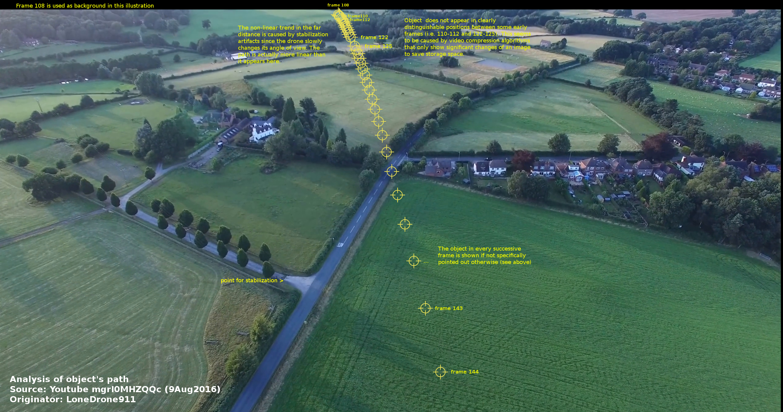
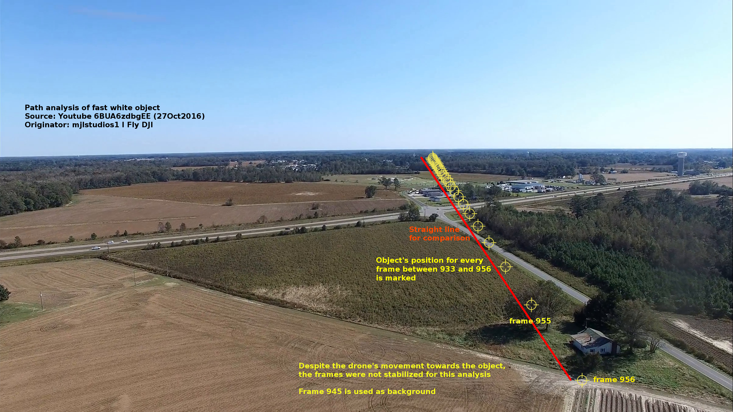
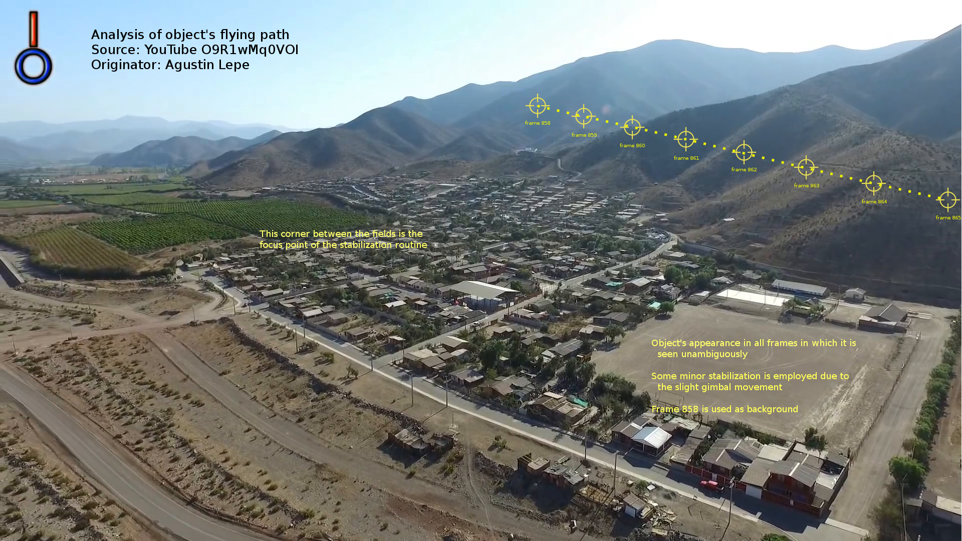
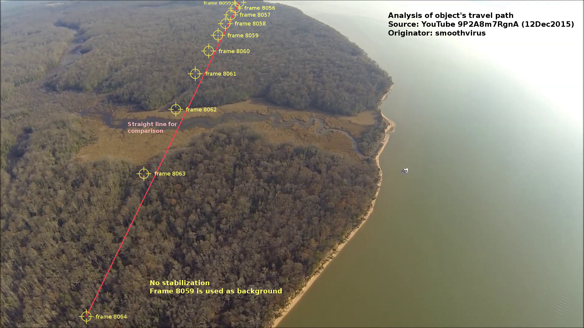
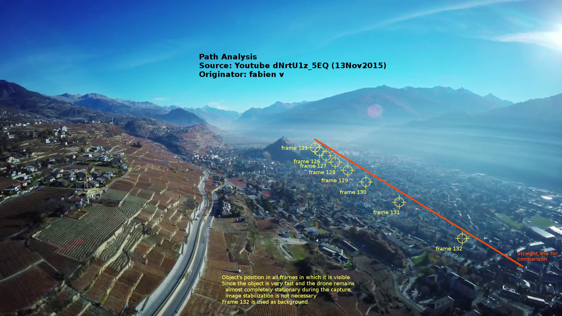
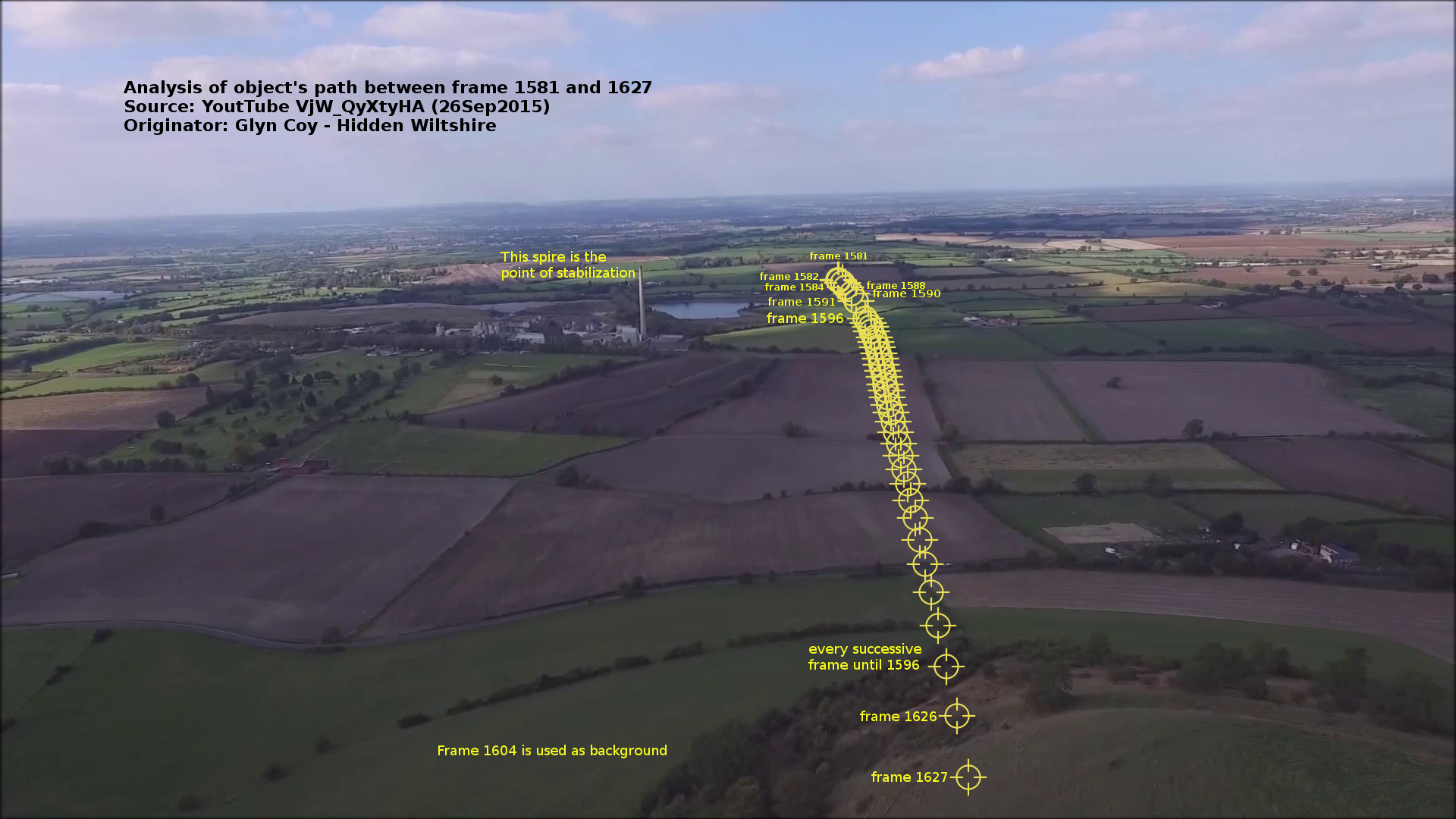
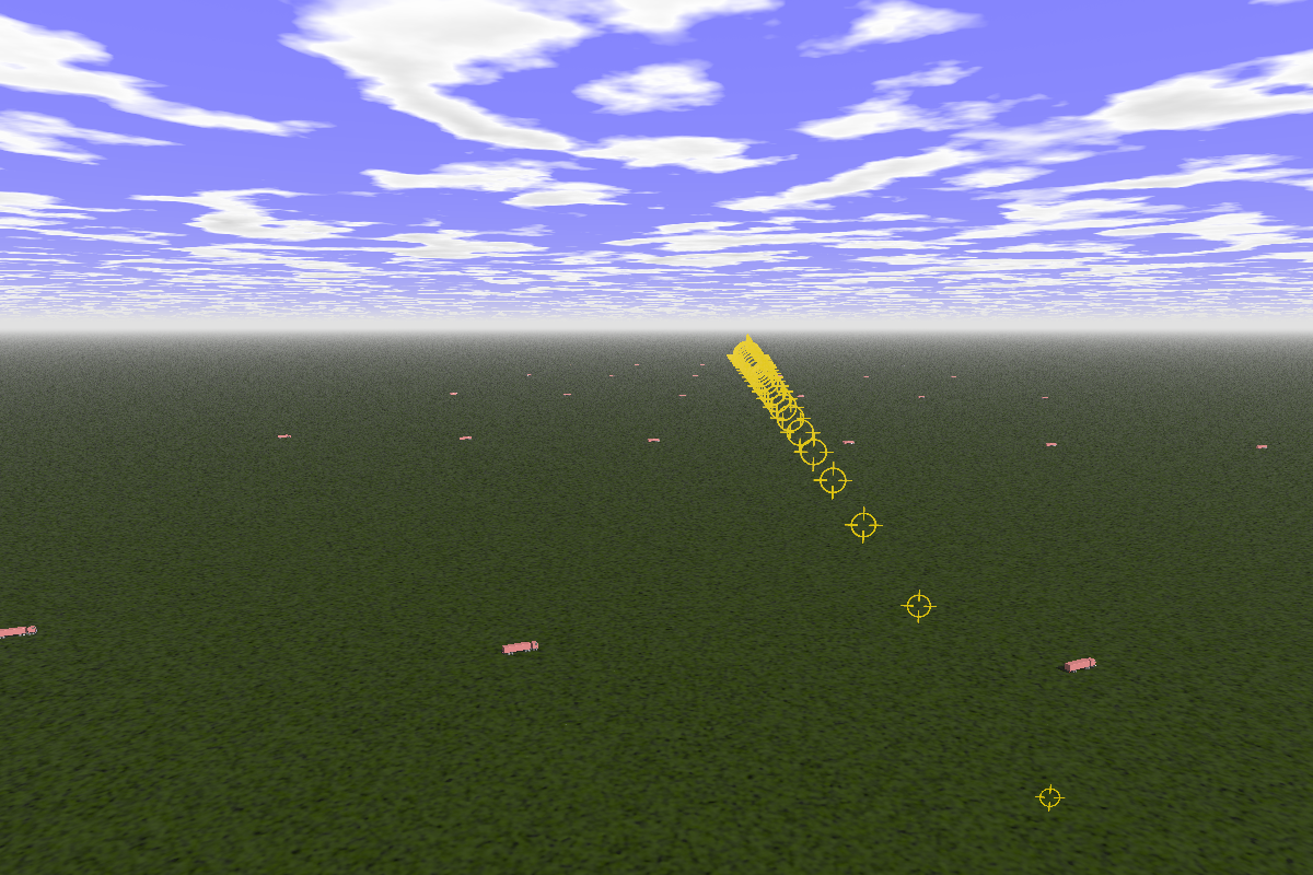
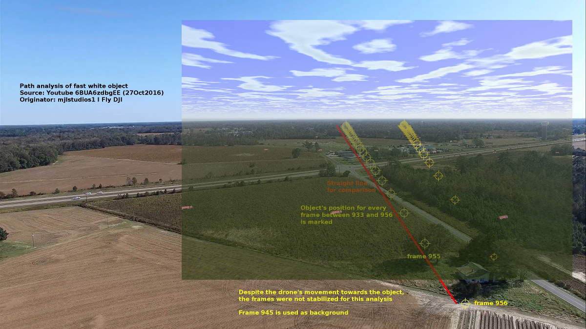 Fig. 8. Case
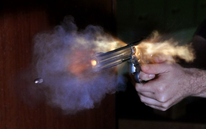 Fig 10. Ultra-high speed photo of a revolver firing. (
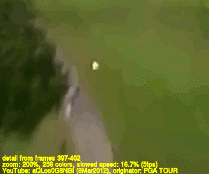
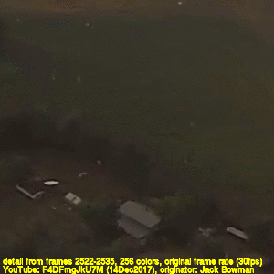 Fig 11. Enlarged and slowed view on near golf ball from figure 1 (left). A drone with a GoPro Hero 3 camera in a hail storm (right,
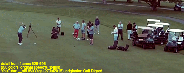